Coordinate Systems and Transformation

Regarding the chart element plotting, compared with setting the appearance properties for a chart element like color and line style, it is more important to specify its position. When plotting a chart, statistical values are used to determine its position. Therefore you will need to create a coordinate system on the canvas according to the chart style, and then transform the statistical values to chart-specific data based on coordinate system settings.

12.2.1 Coordinate systems and axes

esProc provides two commonly used coordinate systems – Cartesian coordinate system and polar coordinate system.

Different coordinate systems have different types of coordinate axes – x-axis and y-axis, or polar axis and radial axis. Each type of axis has its own plotting properties with which the corresponding coordinate transformation operation is handled.

Cartesian coordinate system

A Cartesian coordinate system has two mutually perpendicular axes, denoted the x-axis and y-axis. The logical coordinates on the horizontal x-axis determine the horizontal location of the chart, and those on the vertical y-axis determine the vertical location of the chart. Actually, in a Cartesian coordinate system the abscissa and ordinate of physical coordinates can be calculated individually based on their corresponding logical axes, without any mutual influences.

In all the examples we have cited, the system of Cartesian coordinates is used to position chart elements. The native physical axes on the canvas also belong to a Cartesian coordinate system. The system is used in plotting most of the charts such as column chart, line chart, area chart, scatter chart, bubble chart and stock chart.

Polar coordinate system

The axes in a polar coordinate system are polar axis and radial axis. For the polar axis, you need to define the pole position and the polar axis length; and for the radial axis, the start angle and end angle of the polar coordinates. Conventionally the angle horizontally from the pole to the right is 0 and the counterclockwise angle from the polar axis is positive. By default the start angle of a polar coordinate system is 0 and the end angle is 360.

The system of polar coordinates is used to plot pie chart, doughnut chart, radar chart and etc.

When performing coordinate transformation operation with polar coordinates, a point’s line segment length is calculated from the coordinates on the polar axis and its polar angle is calculated from the coordinates on the radial axis.

12.2.2 Physical axes and logical axes

Physical axes

On a canvas, the prevailing Cartesian coordinate system is the physical coordinate system whose x-axis and y-axis are physical axes, which are fixed and don’t need definition, and generally used to define positions of logical axes.

For physical axes, x-axis runs left to right and y-axis goes up and down. Their coordinate values can be set in proportion or by pixels. 

Ø  Set in proportion

In this case the value range of coordinate x is 0<= x <=1. To set the coordinate system’s position in proportion, place the origin at the top left corner of the canvas and perform calculations in certain proportion to the canvas size. The calculations of abscissas and ordinates will use the canvas’s width or height as the unit size.

Ø  Set by pixels

In this case the value range of coordinate x is x>1 or x<0. When x>1, place origin on the canvas’s top left corner; when x<0, place origin on the canvas’s bottom right corner. To position a chart element by pixels on the canvas, perform calculations according to abscissas and ordinates of the axes as well as the position of origin.

For example, the following plotting algorithm plots a numeric x-axis:

	A
1	=canvas()
2	=A1.plot("BackGround")
3	=A1.plot("NumericAxis","autoCalcValueRange":false)
4	=A1.draw@p(450,350)

As there are no other chart elements to be plotted, set the property of the numeric axis’s Autoclc value range as false, indicating that the value range will not be calculated according to a chart element plotted with this coordinate axis. Default setting will be used to set the position of x-axis:

 

Among properties of the x-axis, by default X start is 0.1, X end is 0.8 and Y position, the vertical distance from the x-axis to the top of the canvas, is 0.8. They are all proportionally defined coordinates on the physical axes, with origin being in the top left corner. In other words, on the canvas the x-axis starts from the 20% length of the width and ends at the 80% length, both from the left; it is located at the 80% length of the height from the top. Below is the plotting result:

In the above figure, the horizontal and vertical unit lengths are respectively 450 pixels and 350 pixels according to the canvas size. For example, that X start is 0.1 means that the distance of start point of x-axis from the canvas’s left-most side is 0.1 times of the unit length 450 pixels, i.e. 45 pixels.

Let’s modify some of the numeric axis’s properties:

X end and Y position are changed to values greater than 1. With the two properties being reassigned, the origin is still located in the top left corner but these two positions will be defined by pixels. Below is the plotting result:

X end is 400, which means the distance of the end point of the x-axis from the canvas’s left-most side is 400 pixels. Setting coordinates on physical axes by pixels makes the plotting more precise but is not so convenient when plotting chart elements whose canvas size is not fixed.

Again let’s modify properties of the numeric axis:

X end and Y position have become negative values. In this case the plotting result would be like this:

When coordinates on a physical axis are negative values, the origin will be in the canvas’s bottom right corner. For example, that the coordinate of X end is -50 means the distance of end point of the x-axis from the canvas’s right-most side is 50 pixels. Actually this is exactly the same chart element as the previous one.

Logical axes

Logical axes are defined by the physical axes. They include numeric axis, enumeration axis, time axis and others. With logical axes, you can calculate the plotting positions from statistical values through coordinate transformation.

For the calculated statistical values, they should be plotted according to a corresponding logical axis. Coordinates of statistical values are referred to as logical coordinates, while the actual coordinates for plotting on the canvas are physical coordinates. By defining the logical axes in the plotting algorithm, you can transform the logical coordinates specified by the chart parameters into physical coordinates when plotting the chart. The physical coordinates under discussion are not the coordinates of the physical axes previously mentioned. Physical coordinates are the actual plotting positions of a chart element on the canvas, whereas the latter refers to coordinates on the native physical axes based on which the logical axes are positioned on the canvas.

For example, the plotting algorithm below defines two numeric axes. “x” is the horizontal axis and “y” is the vertical one:

	A
1	=canvas()
2	=A1.plot("BackGround")
3	=A1.plot("NumericAxis","name":"x","autoCalcValueRange":false)
4	=A1.plot("NumericAxis","name":"y","location":2,"autoCalcValueRange": false)
5
6	=A1.draw@p(350,200)

It produces plotting result as follows:

A5 is added to plot a dot chart:

	A
1	=canvas()
2	=A1.plot("BackGround")
3	=A1.plot("NumericAxis","name":"x","autoCalcValueRange":false)
4	=A1.plot("NumericAxis","name":"y","location":2,"autoCalcValueRange": false)
5	=A1.plot("Dot","axis1":"x","data1":"2","axis2":"y","data2":"6")
6	=A1.draw@p(350,200)

Here are the chart parameters that A5 uses:

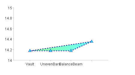
Take the specified x-axis and y-axis as the logical axes for dot chart plotting, and set data for x-axis as 2 and data for y-axis as 6. Then the plotting result is as follows:

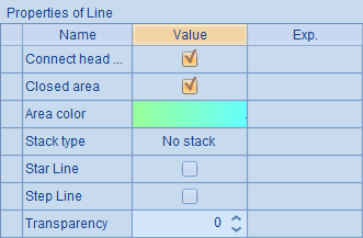
As can be seen, coordinate transformation has been achieved through logical axes. That is, the point is plotted in the required position according to the logical coordinates (2,6) in the dot chart. By default, the grid region on the background of the coordinate system is automatically plotted.

More information about the commonly used logical axes offered by esProc will be covered in Coordinate Axes.