JDBC Enterprise edition

The features explained in this section only supported in esProc Enterprise edition. Users using another esProc edition just skip this section.

Here we introduce how to deploy and use esProc Enterprise edition JDBC. Besides the ordinary esProc JDBC (called PJDBC), we have Enterprise edition JDBC  in esProc Enterprise edition. The two JDBCs are basically same except that they use different esProc related jars. PJDBC uses ordinary esProc related jars while JDBC Enterprise needs Enterprise edition related jars. Same as deploying and configuring the PJDBC, you should deploy the raqsoftConfig.xml file to complete JDBC Enterprise  deployment and, if you want to integrate esProc in a project, you should configure web.xml file in the project.

Downloading, installing and configuring JDBC Enterprise edition

Download esProc Enterprise edition installer in https://www.scudata.com/download-esproc  and install it. After that, find the basic jars used by the Enterprise edition JDBC in [installation directory]\esProc\lib. Different from the other esProc editions, the jar file esproc-ent-xxxx.jar specifically used for the Enterprise edition is necessary. If you want to use the extended functionalities, add the functional jar esproc-ext-xxxx.jar.

Besides [installation directory]\esProc\config\raqsoftConfig.xml, files used to deploy the JDBC Enterprise can also be found in q-server\webapps\qvs\WEB-INF\home. The two configuration files have similar content, but the latter is used for server loading and will not adjust itself when the esProc edition changes. You need to edit it yourself as needed.

Read Scudata Cloud Deployment to find more about esProc Enterprise edition server.

Using JDBC Enterprise edition

Use JDBC Enterprise in the same way as you use PJDBC, such as invoking call statement in Java to execute SPL statement and calling a cellset file. You can use functions unique to the Enterprise edition to perform the operation. Take the following cellset file testQJDBC.splx as an example:

	A
1	=dql("pseudo/test.glmd")
2	=A1.query("select EID, Name, ifMarried from emps")
3	=A2.i()
4	>output(ifpure(A3))
5	return A3

The cellset file uses some functions unique to esProc Enterprise edition. A1 uses dql() function to open a DQL definition file; A2 executes a query statement in DQL; A3 uses P.i() function to convert the result to a pure table sequence where all fields have same data type. To check if the conversion is successful, A4 uses ifpure() function to judge whether it is a pure table sequence or not and output the result.

Use the following Java code to invoke the Enterprise edition JDBC to execute the cellset file. Here we specify configuration file as raqsoftConfig.xml; use the default file if no configuration file is specified:

public void testDataServer(){

Connection con = null;

java.sql.CallableStatement st;

try{

// Establish connection

Class.forName("com.esproc.jdbc.QDriver");

con= DriverManager.getConnection("jdbc:esproc:local://?config=D:/soft/raqsoft/esProc/q-server/webapps/qvs/WEB-INF/home/raqsoftConfig.xml");

// Invoke the stored procedure; createTable1 is the script file name

st =con.prepareCall("call testQJDBC()");

// Execute stored procedure

st.execute();

// Get result set

ResultSet rs = st.getResultSet();

 

// Process result set simply: output field names and data

ResultSetMetaData rsmd = rs.getMetaData();

int colCount = rsmd.getColumnCount();

for ( int c = 1; c <= colCount;c++) {

String title = rsmd.getColumnName(c);

if ( c > 1 ) {

System.out.print("\t");

}

else {

System.out.print("\n");

}

System.out.print(title);

}

while (rs.next()) {

for (int c = 1; c<= colCount; c++) {

if ( c > 1 ) {

System.out.print("\t");

}

else {

System.out.print("\n");

}

Object o = rs.getObject(c);

System.out.print(o.toString());

}

}

}

catch(Exception e){

System.out.println(e);

}

finally{

// Close connection

if (con!=null) {

try {

con.close();

}

catch(Exception e) {

System.out.println(e);

}

}

}

}

The syntax is the same as invoking the ordinary esProc JDBC. Here we use "call testQJDBC()" to execute the SPL file and result is as follows:

Note that dql(), P.i() and ifpure() functions used in this cellset file cannot be used for ordinary esProc JDBC.

Read DQL Tool to find more about esProc Enterprise edition DQL.

esProc Enterprise functions

In the previous section, we mentioned some functions that only work for esProc Enterprise. Here let’s dig a bit deeper into them.

	A	B
1	[Moore,Wilson,Johnson,Smith]	=ifpure(A1)
2	=A1.i()	=ifpure(A2)
3	=demo.query("select EID, NAME, BIRTHDAY from employee")	=ifpure(A3)
4	=A3.i()	=ifpure(A4)
5	=A4.o()	=ifpure(A5)

esProc Enterprise allows using pure sequences. Different from an ordinary sequence, a pure sequence requires same data type for all members. We can use A.i() function to convert an ordinary sequence A to a pure sequence, and use ifpure(A) function to judge whether sequence A is a pure sequence or not. Here are results of A1, B1, A2 and B2:

   

We can see that an ordinary sequence and a pure sequence is displayed in the same way. We can only use the ifpure() function to find whether it is a pure sequence or not.

Similar to a pure sequence, if a field in a table sequence has values of same data type, the field is called the pure field. If a table sequence forces all fields to be pure, it is called a pure table sequence. Note that a pure table sequence uses column-oriented storage. We can use T.i() function to convert an ordinary table sequence T to a pure table sequence, and ifpure(T) function to judge whether table sequence T is a pure one. A pure table sequence and an ordinary table sequence have same appearance, and we can only use ifpure() function to find which type a table sequence is. Here are results of A3, B3, A4 and B4 in the above example:

 

 

We can also use A.o() function or T.o() function to transform pure sequence A or pure table sequence T to an ordinary sequence/table sequence. Below are results of A5 and B5:

 

 

Now let’s look at differences between a pure sequence and an ordinary sequence:

	A	B
1	[Moore,Wilson,Johnson,Smith]	=A1.i()
2	>A1.insert(0,12)	>B1.insert(0,12)

Execute A2 and A1’s data is naturally modified:

A pure sequence requires all its members to have same data type. It does not allow the operation of inserting data of another type or changing the type of a member to another. Therefore, B2’s command in the above code cannot execute and error report will pop up:

The similar thing happens with a pure table sequence:

	A	B
1	=demo.query("select EID, NAME, BIRTHDAY from employee")	=A1.i()
2	>A1(1).BIRTHDAY=20001231	>B1(1).BIRTHDAY=20001231

A2 changes a field value in the first record and data in A1’s table sequence becomes this:

Different from a pure sequence, as each field of a table sequence is a pure sequence, insert and delete commands cannot be used to add or delete records to/from it. If a field value in a table sequence is changed, its data type is required to be keep unchanged. When trying to execute B2, for example, error is reported:

Since there is only one data type across a pure sequence/table sequence, the location operation on it has a noticeably higher efficiency, for example:

	A	B	C
1	=demo.query("select EID, NAME, BIRTHDAY from employee")	=A1.i()	=A1.(NAME)
2	=100000.(C1(rand(500)+1))	=now()
3	=A2.(A1.pselect@1(NAME:A2.~))	=now()	=interval@ms(B2, B3)
4	=A2.(B1.pselect@1(NAME:A2.~))	=now()	=interval@ms(B3, B4)

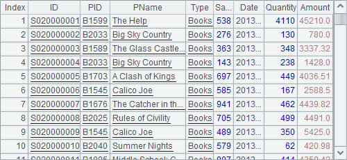
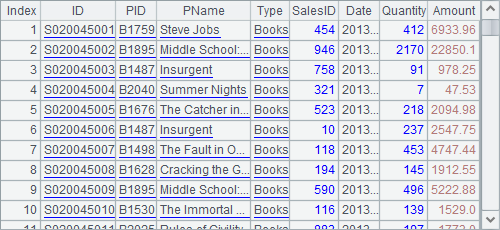
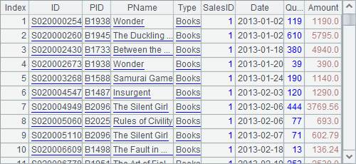
A1 is an ordinary table sequence; B1 is a pure table sequence. A2 generates 100,000 NAME values randomly. A3 and A4 respectively get position of each NAME value from EID field of the ordinary table sequence and the pure table sequence. Results of them are same:

 

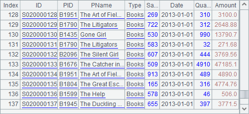
C3 and C4 find and compare the time spent for performing the location. It can be seen that it takes a far shorter interval of time to find the target data in the pure table sequence:

 

One thing you need to remember: data in a pure table sequence is stored column-oriented, and a record needs to obtain its data from each column according to positions. Therefore, performance is compromised even though the location is fast.

	A	B	C
1	=demo.query("select EID, NAME, BIRTHDAY from employee")	=A1.i()	=A1.(NAME)
2	=100000.(C1(rand(500)+1))	=now()
3	=A2.(A1.select@1(NAME:A2.~))	=now()	=interval@ms(B2, B3)
4	=A2.(B1.select@1(NAME:A2.~))	=now()	=interval@ms(B3, B4)

In this example code, A3 and A4 use the select function T.select() instead of the location function T.pselect(), and both return a same record sequence consisting of records. Difference is that records in A4’s result set all come from the pure table sequence. A record sequence made up of records of a pure table sequence is called pure record sequence. It needs to get data from every column to be displayed:

 

C3 and C4 find and compare the time intervals spent for performing the two types of data selection, and return the following results:

 

In this case, the pure table sequence has no advantage at all. So, we should choose to use the pure sequence/table sequence according to real-world situations.

 

Usually, every field of a table queried from the database has same data type. db.query(sql) function can work with @v option to directly return result as a pure table sequence:

	A	B
1	=demo.query@v("select EID, NAME, BIRTHDAY from employee")	=ifpure(A1)
2	=A1.select(left(NAME,1)=="J")	=ifpure(A2)
3	=A1.select@v(left(NAME,1)=="J")	=ifpure(A3)
4	[Rebacca, Matthew, Smith]
5	=A4.(A1.select@v(NAME==A4.~)).conj()	=ifpure(A5)
6	=A4.(A1.select@v(NAME==A4.~)).conj@v()	=ifpure(A6)
7	=A6.sort@v(BIRTHDAY)	=ifpure(A7)

Here are results of A1 and B1:

 

T.select(sql) function returns a pure record sequence, which is an ordinary sequence consisting of records coming from a pure table sequence, when it performs a computation on a pure table sequence. It can work with @v option to return a pure table sequence. Similarly, we can use A.select@v(…) on pure sequence A to get a pure sequence. Here are results of A2, B2, A3 and B3:

 

 

By default, the result of concatenating multiple pure sequences is an ordinary sequence. We can also use @v option in A.conj(…) function to get a pure table sequence. Here are results of A5, B5, A6 and B6 in the above piece of code:

 

 

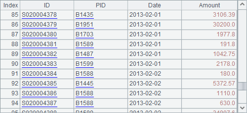
We can also use T.sort@v(…) function and P.sort@v(…) function to sort records of pure table sequence T or pure record sequence P and return result as a pure table sequence. Here are results of A7 and B7:

 

 

T.new(…) function and T.derive(…) function will still return a pure table sequence when generating a new table sequence from a pure table sequence. And by using @o option in it, we can make use of the existing columns in the table to increase efficiency. For example:

	A	B	C
1	=demo.query@v("select NAME, SURNAME, STATE, DEPT from employee")
2	=1000.(A1).conj@v()	=now()	=ifpure(A2)
3	=A2.new(#:ID, NAME/" "/SURNAME:FullName, STATE, DEPT)	=now()	=ifpure(A3)
4	=A2.new@o(#:ID, NAME/" "/SURNAME:FullName, STATE, DEPT)	=now()	=ifpure(A4)
5	=interval@ms(B2,B3)	=interval@ms(B3,B4)
6	>A2(1).NAME = "New Name"	>A2(1).STATE = "New State"

A1 has relatively a small amount of data, and A2 copies it for 1,000 times before generating a pure table sequence, whose data is as follows:

Both A3 and A4 use T.new(…) function to generate a new table sequence. Difference is that A4 uses @o option to enable the use of the existing columns in A2 to generate a new pure table sequence. In order to do this, line 6 modifies the NAME field and STATE field of A2’s first record. After execution, A3 and A4 generate new table sequences as follows:

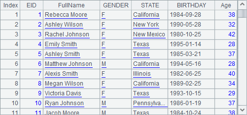
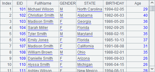
Though the original table sequence A2 is modified after the new table sequences are generated, STATE field of the first record in A4’s result set is also changed, according to the above results. This is because A4 shares the STATE field with A2. Yet, since A4’s FullName field is newly-generated, it is not affected by the change of A2’s NAME field. Besides, A3 does not use @o option, and it is also not affected by the data modification.

According to results of C2, C3 and C4, A2, A3 and A4 are all pure table sequences:

  

And according to the time intervals obtained by A5 and B5, the use of @o option brings much higher efficiency.

 

QVS and QJDBC

Once esProc Enterprise is installed, there is the complete QVS project, also known as esProc Enterprise Multifunction Server, under the product’s installation directory. The specific directory where the project is accommodated is [installation directory]\esProc\q-server. In [installation directory]\esProc\q-server\lib, there are basic jar files used by the esProc Enterprise and QJDBC. Apart from these, you also need ecloud-xxxx.jar to deploy cloud storage functionality for the esProc Enterprise.

The QVS startup file is StartQVS.bat (StartQVS.sh under Linux), which is located in [installation directory]\esProc\bin. The local QVS server will by default automatically started. Go to Scudata SPL Cloud Deployment to learn more or change the existing configurations. Below is the QVS interface after it is successfully started:

QJDBC is the JDBC Enterprise with QVS functionality built in. Its driver class is com.esproc.jdbc.QDriver, and the URL is jdbc:esproc:q:local://. You can directly use the following functions when QJDBC is started.

	A
1	=Qconnect("http://localhost:8090/qvs":"demoqvs",30,300)
2	=Qdirectory("test/")
3	=Qfile("test/cities.txt")
4	=A3.import@t()
5	=Qenv("arg1", "Sale")
6	=Qenv("arg1")
7	=A1.exec@x("test/FindEmployees1.splx";A6)
8	>A1.close()

A1 executes Qconnect(url:v, wt, it) to connect to the QVS server in the specific URL; the verification is demoqvs, the maximum wait time is 30 seconds and the maximum idle time is 300 seconds. Once connected, it can perform remote services.

A2 uses Qdirectory(path) function to get a list of names of all files under the specified path.

A3 uses Qfile(fn) function to retrieve the specified file and return a file object. Then we can further compute it, such as importing data of the file into a table sequence.

A5 uses Qenv(name, value) function set up a global variable, and A7 reads the global variable.

	A
1	$(demo) select * from EMPLOYEE where DEPT = ?;arg1
2	>output("before return")
3	return A1

A7 uses A1’s connection object to execute the splx cellset file. It uses A6’s value as the query parameter, and A8 closes the connection. Below is the query result of A7:

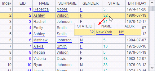
The Qconnect(), Qdirectory(), Qfile() and Qenv()used in the above example code are functions for executing QJDBC. They also called Q functions. The other Q functions supported by QJDBC are Qmove(), Qload() and Qlock(). Go to Function Reference to learn more about them.

In addition to using a Q function to access QVS, we can also employ the remote server in esProc Enterprise. Find more related content in Deploy and Use RSRV in esProc Enterprise Edition.