Process Data
After a data source is imported into the ETL file, you can perform operations on it, such as adding computed column, filtering, sorting, grouping & aggregation, retrieving fields, set operations and data association.
Add Computed Columns
This item is used to add computed columns to the current data source and generate a new data set.
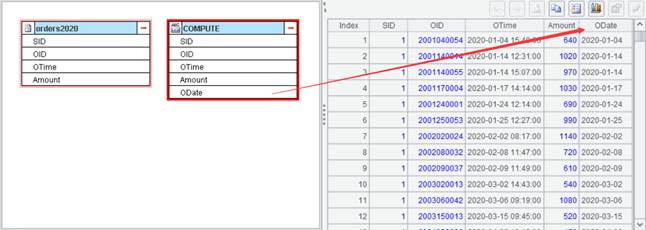
For example, to import text file orders2020.txt and add a new column named ODate to source data orders2020 by computing expression date(OTime) on OTime field:
Select the data source, click Edit -> Add Computed
Columns or Add Computed Columns icon ![]() on the toolbar to enter the
following interface, and then icon
on the toolbar to enter the
following interface, and then icon ![]() to edit the computed column expression:
to edit the computed column expression:

Parallel computation: Use parallel processing to enhance performance of data-intensive complex computations. The order of parallel computations is not fixed.
Then click OK and a new data set is generated, as shown below:
Select Fields
This item is used to compute expressions on certain fields of the source data and generate a new data set.
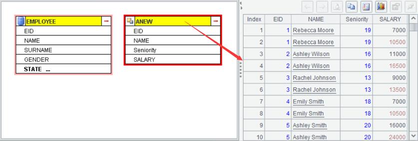
Example: Import database table EMPLOYEE; the result type is cursor. Select fields EID, NAME, SURNAME, HIREDATE and SALARY from cursor type source table EMPLOYEE, concatenate NAME field and SURNAME field into NAME field, compute the hire duration based on HIRDATE field and generate Seniority field, and generate a new data set where each EID corresponds to two pieces of data – the original SALARY and the increased SALARAY by 50%.
Click Edit -> Select Fields, or Select Fields icon ![]() on the toolbar to make the following
configurations:
on the toolbar to make the following
configurations:
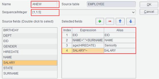
Sequence/Integer: Optional. Suppose the content to-be-entered is parameter X, which can be a sequence or an integer, then in the expressions under Select Fields, you can use “~” to reference X. When it is an integer, it can be understood as to(X), which means performing X rounds of computations on the result set.
Click OK to generate a new data set:
Filter
This item computes the filtering expression on data in the data source to select records meeting the specified conditions and generates a new data set.
Example: Import database table EMPLOYEE; the result type is cursor. Set filtering conditions on the table sequence type source data EMPLOYEE and select records whose DEPT is sales and whose SALARY is greater than 5,000.
Select the data source, click Edit -> Filter
or Filter icon ![]() on the toolbar to enter the Filter
interface, where you edit filter expression DEPT
== "Sales" && SALARY > 5000, as
shown below:
on the toolbar to enter the Filter
interface, where you edit filter expression DEPT
== "Sales" && SALARY > 5000, as
shown below:

Click OK to generate a new data set:

In a filter expression, you can use operators as well as the esProc functions. For example, to perform filtering on the above FILTER data set to select records of employees whose names begin with letter B, the filter expression is like(NAME,"B*") and the configurations are as follows:

Click OK to generate a new data set:

Sort
This item specifies the sorting field and sorting direction for sorting data in the data source and generates a new data set using the sorted data.
Example: Import text file orders2020.txt and sort source data orders2020 by SID field in descending order and by Amount field in ascending order.
Select the data source, and click Edit -> Sort or Sort
icon ![]() on the toolbar to enter the
Sort interface, where you click Add button
on the toolbar to enter the
Sort interface, where you click Add button ![]() to add a sorting field, as shown below:
to add a sorting field, as shown below:

Ascending: Sort data in ascending order. A cursor type result set only supports the ascending order.
Parallel computation: Use parallel processing to enhance performance of data-intensive complex sorting operations. A cursor type result set does not support this option.
Place null values in the end: Put records where the sorting field values are null in the end.
Click OK to generate a new data set:
Group
The item groups and summarizes a data set and generates a new data set using the computed data.
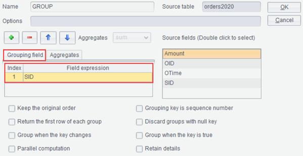
Example: Import text file orders2020.txt, group source data orders2020 by SID field, and find the number of OIDs and sum Amount values in each group.
Select the data source, and click Edit -> Group or Group
icon ![]() on the toolbar to enter the
Group interface, where you add a grouping field and the field to be aggregated,
as shown below:
on the toolbar to enter the
Group interface, where you add a grouping field and the field to be aggregated,
as shown below:

Do not sort result set by grouping field: The result set won’t be sorted by the specified grouping field when it is selected.
Grouping key values are ordinal numbers: Directly locate the target data when grouping key value is an ordinal number.
Return the first row of each group: By default, return records of the current group. When Retain details is also checked, get the first record from each group, concatenate them to return, while ignoring the other options.
Discard a group whose members are null: If result of the grouping field expression matches none, discard the group whose members are null.
Create a new group when grouping key changes: Group records by comparing each with its next one, which is equivalent to a merge, and do not sort the result set.
Create a new group when grouping key is true: Create a new group whenever the result of computing the grouping field expression is true.
Parallel computation: Use parallel processing to enhance performance of data-intensive complex grouping operations.
Retain details: Add a new details field to store record of each group before aggregation.
Click OK to generate a new data set:

Pivot
This item is used to transpose rows to columns or columns to rows in a data set.
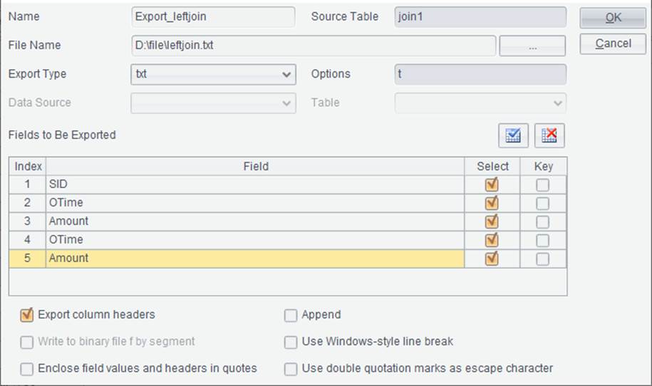
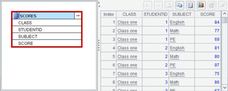
Example: Import database table SCORES, and perform row-to-column transposition on SUBJECT field values in source table SCORES. Below is data set SCORES:
Select
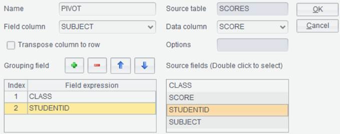
the data source, click Edit -> Pivot or Pivot icon ![]() to enter Pivot interface, where
you set CLASS and STUDENTID as the grouping fileds and New Column Names as SUBJECT and Detail Data Column as SCORE:
to enter Pivot interface, where
you set CLASS and STUDENTID as the grouping fileds and New Column Names as SUBJECT and Detail Data Column as SCORE:
Transpose column to row: Perform column-to-row tansposition on the result set.
Click OK to generate a new data set:

Set Operations
This item is for performing intersection, union, concatenation and difference operations on multiple data sets.
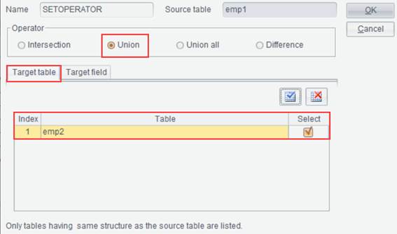
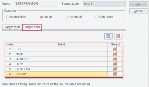
Example: Import bin files emp1.btx and emp2.btx and compute their union. Here are emp1 and emp2 data sets:

Select one of the data sets, like emp1, and click Edit -> Set
Operations or Set Operations icon ![]() on the toolbar to pop up Set
Operations interface, where you select Target Table, Operator
and Target Field, as shown below:
on the toolbar to pop up Set
Operations interface, where you select Target Table, Operator
and Target Field, as shown below:

Click OK to generate a new data set:
Join
The item is used to associate multiple data sets through the joining field.
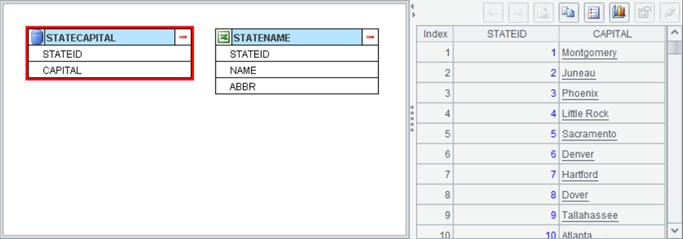
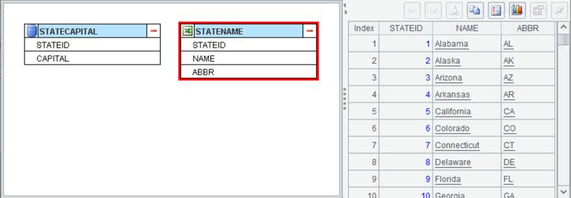
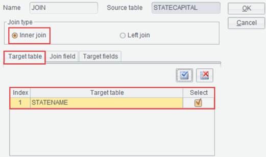
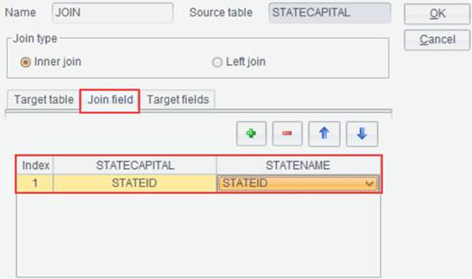
Example: Import database table STATECAPITAL and Excel file STATENAME.xlsx and perform an inner join between the two data sets according to STATEID. Here are data sets STATECAPITAL and STATENAME:

Select one of the data sets, like STATECAPITAL, and click Edit ->
Join or Join icon ![]() on the toolbar to pop up the Join interface,
where you select Target Table, Join Type, Join Field and Target
Fields, as shown below:
on the toolbar to pop up the Join interface,
where you select Target Table, Join Type, Join Field and Target
Fields, as shown below:

Click OK to generate a new data set:
Edit Parameters
You can use parameters in expression for data processing.
Example: Perform a filtering operation on source table EMPLOYEE to select records whose DEPT is the specified value. In this case a parameter can be used to represent the specified value.
Parameter settings: Click Tool -> Edit
Parameters to enter the Edit Parameters interface, where you click Add
button ![]() to add a parameter:
to add a parameter:

Add parameter arg1 and assign value to it, then you can use the parameter in expression. Select source table EMPLOYEE, click Filter and edit the Filter Expression:

Click OK to generate a new data set:
