Accessing a (multi-zone) composite table

The f. open() function is used to open a composite table saved as a file:

	A	B
1	=file("D:/file/dw/employees.ctx")
2	=A1.open()	=A2.cursor().fetch()
3	=A2.attach(stable)	=A3.cursor().fetch()
4		=A3.cursor(EID,Dept,Gender,Name,OCount,OAmount).fetch()
5	>A2.close()

A2 opens the composite table’s base table with f.open() function where the parameter is absent. In A3, T.attach function opens an attached table by specifying its name. B2 retrieves data from the composite table’s base table:

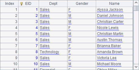
The retrieved data is the data populated to the composite table, where EID is the primary key.

B3 retrieves data from the attached table stable:

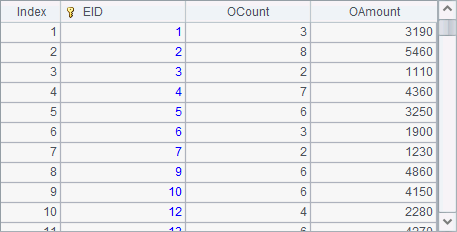
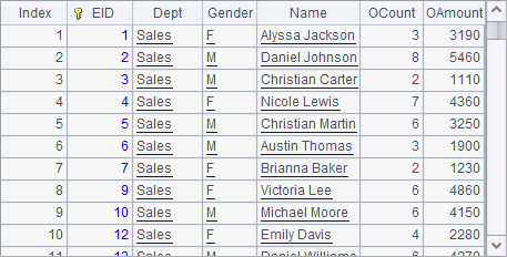
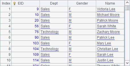
The data retreived from an attached table can contain fields of the base table. B4, for example, retrieves data containing fields of the base table while generating a cursor:

In the above, T.cursor() function is used to retrieve data from entity table. We can also use T.cursor(C₁, C₂…; w) function to specify the fields we want through parameters C₁, C₂… or the records we desire using a query condition w when retrieving data from an entity table:

	A	B
1	=file("D:/file/dw/employees.ctx")
2	=A1.open()	=A2.attach(stable)
3	=A2.cursor(EID,Name,Dept)	=A3.fetch()
4	=A2.cursor(;right(Name,1)=="e")	=A4.fetch()
5	=B2.import(EID,Name,OCount,OAmount;OAmount>5000)	>A2.close()

A3 retrieves only three fields from the base table. B3 fetches data as follows:

A4 specifies a query condition, which is getting records where the employee names end with letter e. Here’s B4’s result:

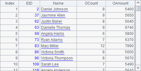
To retrieve all eligible data from the entity table, you can use T.import(C₁, C₂…; w) function. A5 retieves from stable the order records where OAmount is greater than 5000. Here’s B5’s result:

When a composite table contains a large amount of data, we can perform segmental retrieval. But first we need to split the composite table and store it by segment. We need to specify the field according to which the entity tables in a composite table are split when segmental storage is needed. Let’s look at how to store data in and retrieve data from an enity table by segment:

	A	B
1	=file("D:/file/dw/employees.ctx")	=A1.open()
2	=B1.attach(stable)
3	=file("D:/file/dw/orders.ctx")	=A3.open()
4	=B3.attach(otable)
5	=A2.cursor(;;1:3).fetch()	=A2.cursor(;;2:3).fetch()
6	=A4.cursor(;;1:3).fetch()	=A4.cursor(;;2:3).fetch()
7	>B1.close()	>B3.close()

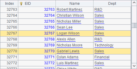
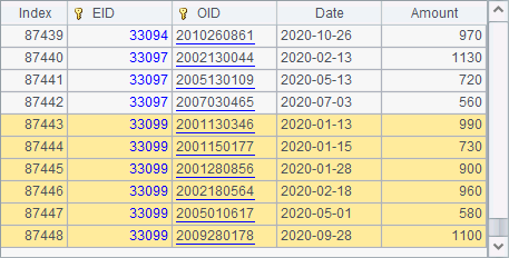
A2 retrieves the attached table stable from the composite table file employees.ctx. Both A5 and B5 retrieve one segment of stable from 3 segments. A5 retrieves the first segment and B5 retrieves the second segment. Below are the retrieved segments:

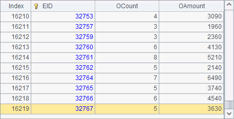
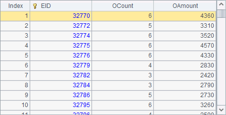
By comparing the results with A4’s employee data in the previous example, we find that the last seller ID in the first segment, 32767, and the first seller ID in the second segment, 32770, are neigbours. This shows the segmental retrieval traverses and reads all records only once.

A4 opens the attached table otable. Both A6 and B6 retrieve one segment of otable from 3 segments. A6 retrieves the first and B6 retrieves the second. Below are the retrived segments:

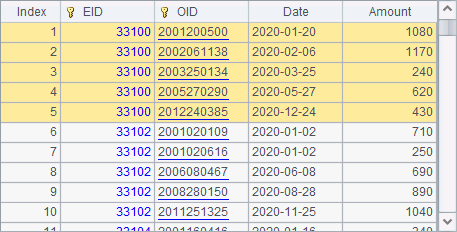
Because otable is a large table, the records in each segment is a lot more. As the composite table orders.ctx is stored by segment by EID, records of the same seller will be put into one segment. Thus the last record of one segment and the first record of the next segment belong to different seller. Comparing the two segments with those retrieved in B5 and B6, we find that records in corresponding segment in two composite tables are different. For example, EID in the second segment’s first record in employees table is 32770 while EID in the second segment’s first record in orders table is 33100.

When the computation involves entity tables in different composite tables, we use multicursor to ensure the synchronization of their segmentation:

	A	B
1	=file("D:/file/dw/employees.ctx")	=file("D:/file/dw/orders.ctx")
2	=A1.open()	=B1.open()
3	=A2.attach(stable)	=B2.attach(otable)
4	=A3.cursor@m(;;3)	=B3.cursor(;;A4)
5	=joinx(A4:s,EID;B4:o,EID)	=A5.fetch()
6	=A3.cursor@m(;;3)	=B3.cursor(;;A6)
7	=joinx(A6:s,EID;B6:o,EID)	=A7.groups(s.EID:EID;count(~):Count, sum(o.Amount):Sum)
8	>A2.close()	>B2.close()

A3 and B3 retrieve two entity tables stable and otable repectively from two composite tables. In A4, T.cursor@m(;;n) function splits stable into n segments to generate a multicursor. B4 splits entity table otable according to A4’s multicursor. Then in A5, joinx function joins the synchronized multicursors in A4 and B4. Here’s the join result in B5:

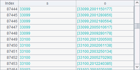
According to the same way of segmentation, segments in the two cursors match completely.

B7 re-generates multicursors to calculate number of orders and sales amount for each seller:

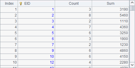
A comparison with stable’s OCount and OAmount fields in the above shows the joining result is correct.

Since an entity table can be retrieved in segments, the cs.joinx(C:…, T:K:…, x:F,…;…;n) function also applies to it. In the function, entity table T replaces the segmentable bin file f to join with data in a cursor.

We can create an index for an entity table according to a certain condition. An index-based query will be much more efficient. For example:

	A	B
1	=file("D:/file/dw/employees.ctx")	=A1.open()
2	=B1.import(;)
3		=now()
4	=B1.cursor(;[8136,11247,83372,264,8223,826, 32758,1341,6255,1983].contain(EID))	=A4.fetch()
5		=interval@ms(B3, now())
6	=B1.index(file("D:/file/dw/idx"), [8136,11247,83372,264,8223, 826,32758,1341,6255,1983].contain(EID);EID)	=now()
7	=B1.icursor(;[8136,11247,83372,264,8223,826,32758,1341, 6255,1983].contain(EID);file("D:/file/dw/idx"))	=A7.fetch()
8		=interval@ms(B6, now())
9	>B1.close()

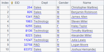
Line 1 and line 2 open the base table, or the entity table employees, in the composite table employees.ctx. Line 4 queries the corresponding 10 records in employees. B4 fetches the records as follows:

In A6, T.index(f:h,w;C,…;F,…) function creates an index file named idx on indexed field EID for employees. In A7, T.icursor(C,…;w;f,…) function performs query according to the index file. B7 gets the same result as B4 does.

B5 and B8 calculate how long it takes the two methods to query the 10 records:

 

An index makes the query faster. So, it can also speed up a query over a row-based composite table.

If the key of a composite table is a serial byte field, we can use a part of the key value as the segmenting condition. This offers us more information through the key and increase efficiency. For example:

	A	B	C	D
1	=file("D:/file/dw/students.ctx")	=create(ID,City,School, SID)
2	for 20	="C"/A2	=20+rand(31)
3		for C2	=B2/"_S"/B3	=rand(4001)+1000
4			for D3
5				>B1.insert(0,k(A2,B3,C4:2),B2,C3,C4)
6	=A1.create@y(#ID,City, School,SID)	>A6.append(B1.cursor())	=A1.open()
7	=A6.import(;;10: 200)	=A6.import(;;11: 200)	>A6.close()

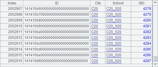
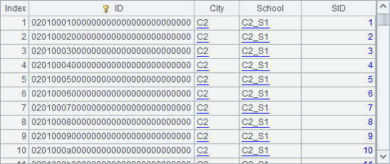
From line 2 to line 6, data for the composite table is generated and stored in B1’s table sequence. The data consists of several fields – ID, City, School and SID, and includes students records from 20 cities, which are C1~C20. Each city includes 20~50 schools, and each school has 1000~5000 students. The ID field contains serial byte data where valid information is stored in the first four bytes. The first byte is city code, the second is school code, and the third and the fourth are student ID. Note that one byte’s value range is 0~255, and two bytes’ is 0~65535. Every type of data should get its value within its range. Here is B1’s data:

A6 creates the composite table’s base table and populates data to it.

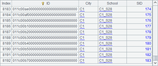
Here’s data in A7:

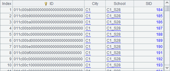
Data in B7:

Records in two neighboring segments could belong to same city or school, which is inconvenient to use in the computation. So, we can store data in a composite table in different files as needed, for instance:

	A	B
1	=file("D:/file/dw/students.ctx")	=A1.open()
2	=file("D:/file/dw/students.ctx":to(20))	=B1.create(A2; int(ID.sbs(1)}))
3	=B1.cursor()	>B2.append@x(A3)
4	=file("D:/file/dw/students.ctx":2)	=A4.open()
5	=B4.cursor().fetch(100)	>B4.close()
6	=file("D:/file/dw/students.ctx":3)	=A6.open()
7	=B6.cursor().fetch(100)	>B6.close()
8	>B1.close()

In A2, file(fn:zs) function generates a homo-name files group. Parameter fn is the file name, and parameter zs is an integer sequence. If there are n integers in the integer sequence, n files will be generated for the homo-name files group. A composite table generated from a homo-name files group is called a multi-zone composite table, where each member is a zone table that can be accessed separately through the corresponding zone name and zone table number. A2 uses 20 zone tables that correspond to 20 cities. B2 uses T.create(fg; x) function to generate a multi-zone composite table according to the structure of composite table students.ctx in the previous example. Parameter fg is a homo-name files group, and parameter x is a zone table expression whose result is an integer referring to a certain zone table. We can also use fg.create(C₁,C₂,…; x) function to generate a multi-zone composite table. B2 gets city codes through serial byte type IDs and uses them as zone table numbers.

B3 writes A3’s cursor data to B2’s multi-zone composite table. @x option is used because the cursor data that comes from the composite table generated by the previous cellset file could correspond to more than one zone table. At each append, a zone table expresson is computed to check whether the data originates from the corresponding zone table. If data to be appended to a multi-zone composite table belongs to a multicursor, each part of the cursor corresponds to only one zone table, and there is no need to compute zone table expressions.

In A4, file(fn:z) function gets one zone table file named students.ctx and numbered 2. According to the specified zone table expression, the zone table stores data of the second city. A5 fetches data from B4’s cursor and gets the following result table:

Similarly, A6 gets the third zone table, and A7 fetches data from its corresponding cursor as follows:

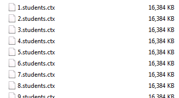
As we can see, a multi-zone composite table stores data in a group of numbered homo-name files (as shown below), which is called a homo-name files group. The storage is efficient, and file access and management of are convenient. In this example, students.ctx represents an ordinary composite table while a multi-zone composite table consists of a set of zone tables whose names are made up of zone table number plus students.ctx. Below is a multi-zone composite table file stored in a folder:

If a composite table can associate with an existing records sequence or a cursor, we can use T.new(A/cs, x:C, …:w) function, T.derive(A/cs, x:C, …;w) function or T.news(A/cs, x:C, …;w) function to get another or certain other fields from entity table T according to matching condition w and generate a new table sequence/cursor, or add a new field and then generate a new table sequence/cursor. For example:

	A
1	=file("D:/file/dw/employees.ctx")
2	=A1.open()
3	=create(EID,Salary).keys(EID).record([1,10000,147,12000,179,9800])
4	=A2.new(A3, EID, Dept, Name, Salary)
5	=A2.derive(A3.cursor(), Dept, Name; Dept=="Sales").fetch()
6	>A2.close()

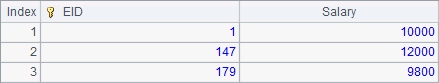
A3 creates a new table sequence consisting of primary key EID and Salary field and to which three records are inserted:

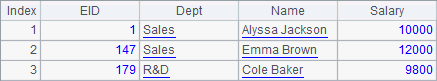
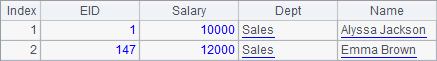
A4 uses T.new(A/cs, x:C, …:w) function generates a new table sequence by getting EID field, Dept field, Name field and Salary field from A2’s table sequence. Among the four fields, Dept and Name come from composite table employees.ctx. A specific function operation will query records in a composite table’s entity table to get matching ones according to the primary key of A3’s table sequence and retrieve values of certain fields. Note that the specified table sequence’s primary key must be ordered by the entity table’s primary key. Below is A4’s result:

A5 uses T.derive(A/cs, x:C, …:w) function to get data from the composite table’s entity table to generate a new field. A cursor-based operation will return a cursor, too, and fetch() function is needed to get data from the result set. A filtering condition is specified to get records of employees of sales department. Below is the result:

Both T.new(A/cs, …) function and T.derive(A/cs, …) function allows data in the specified table sequence or cursor come from somewhere eles instead of the composite table that entity table T belongs to. The data retrieval is performed only by matching their primary keys.

With T.news(A/cs, …) function, entity table T is generally the subtable of table sequence A or cursor cs. Each record in the table sequence or cursor corresponds to multiple records in the entity table, and thus multiple records will be accordingly generated in the new table sequence. In this case the entity table has more than one primary key while the table sequence or the cursor’s primary key corresponds to only one or some of the keys.