Associating Tables by the Foreign Key

In relational databases the foreign key is often used to identify the relationship between tables. In esProc the relationship of correspondence between tables can also be expressed by the foreign key.

3.5.1 Foreign key field

A.derive() function is used in esProc to add one or more columns to a record sequence. For example:

	A
1	=demo.query("select EID, NAME, SURNAME, BIRTHDAY from EMPLOYEE")
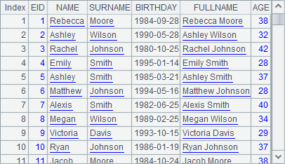
2	=A1.derive(NAME+" "+SURNAME: FULLNAME, age(BIRTHDAY):AGE)

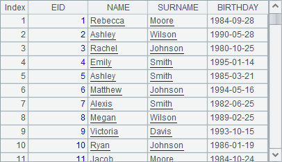
A1 retrieves employee information. A2 adds computed columns - FULLNAME and AGE - to A1’s table sequence, returns a new table sequence, and computes the employees’ full names and ages.

Below is the table sequence in A1:

With the computed columns added, A2 gets a new table sequence as follows:

After learning how to add computed columns to a table sequence, we’ll explore the link between the computed columns and creating relationship between tables.

Often relationships exist between two database tables. In esProc the relationship can be expressed by directly referencing the records of a table sequence by another one, making the data search and presentation simple and the data structure clear.

Using A.derive() function, you can add columns to a table sequence and make the data type of the values the records or the record sequences referenced from another table sequence, creating the foreign key for linking the two tables. For example:

	A
1	=demo.query("select * from CITIES")
2	=demo.query("select STATEID, NAME, ABBR, CAPITAL from STATES")
3	=A1.derive(A2.select@1(STATEID==A1.STATEID):State)
4	=A3.derive(State.ABBR:SA)
5	=A2.derive(A1.select(STATEID==A2.STATEID):Cities)

A1 and A2 retrieve data from the database tables - CITIES and STATES - respectively:

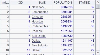
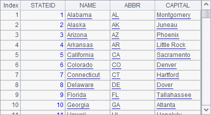
The CITIES table is related to the STATES table through STATEID field. This kind of storage pattern in databases can keep data consistency, make data easy to maintain and, at the same time, save storage spaces.

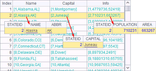
A3 adds a State field to CITIES to create a foreign key for storing the records of states in which cities located. For the convenience of later check, A4 continues to add an SA field to CITIES to list abbreviations of these states. A5 adds a Cities field to STATES as the foreign key for storing records of cities in every state.

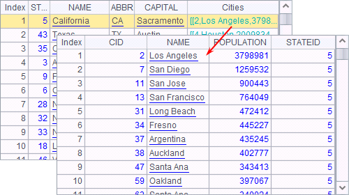
Execute the program and the data of A4 is as follows:

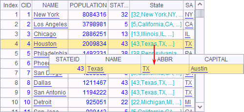
In the above, the State field contains records of states. You can double-click a value to see details.

Data of A5 is as follows:

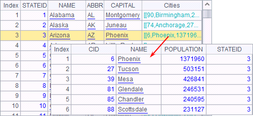
The Cities field contains records of cities in each state. Double-click each value to see details.

Through creating foreign keys, both table sequences of A4 and A5 have obtained all information of the two original tables: STATES and CITIES, in the database; relationship between the two tables is established. Note that the data types of these foreign key fields are different. The foreign key State in A4 is record data type while the foreign key Cities in A5 is record sequence (i.e. a sequence of records) data type.

Actually the STATEID field in the STATES table is usually the primary key, through which a second table, like CITIES, can be linked to it using the switch function. For details about the function, refer to Primary Key and Index.

3.5.2 Using foreign key

A foreign key field is treated as any other field during querying or presenting data of a table sequence. But you need to pay attention to the data type it uses.

For example, to select from the CITIES table the cities that are located in the states whose names contain “la”, you can directly call the NAME field of the foreign key State in the filtering expression:

	A
1	=demo.query("select * from CITIES")
2	=demo.query("select STATEID, NAME, ABBR, CAPITAL from STATES")
3	=A1.derive(A2.select@1(STATEID==A1.STATEID):State)
4	=A3.derive(State.ABBR:SA)
5	=A2.derive(A1.select(STATEID==A2.STATEID):Cities)
6	=A4.select(like(State.NAME,"*la*"))

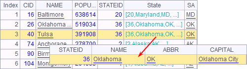
Note that here the data type of the foreign key field is record. The result of A6 is as follows:

A foreign key field can also be used as the sorting criterion, like sorting the states data in descending order according to the number of cities in a state:

	A
1	=demo.query("select * from CITIES")
2	=demo.query("select STATEID, NAME, ABBR, CAPITAL from STATES")
3	=A1.derive(A2.select@1(STATEID==A1.STATEID):State)
4	=A3.derive(State.ABBR:SA)
5	=A2.derive(A1.select(STATEID==A2.STATEID):Cities)
6	=A5.sort(-Cities.len())

Note that here the data type of the foreign key field is record sequence. The sorting result of A6 is as follows:

If the records referenced by a foreign key field of a table sequence also contain a foreign key field, they still can be referenced. For example, listing the cities whose states happen to contain three cities:

	A
1	=demo.query("select * from CITIES")
2	=demo.query("select STATEID, NAME, ABBR, CAPITAL from STATES")
3	=A2.derive(A1.select(STATEID==A2.STATEID):Cities)
4	=A1.derive(A3.select@1(STATEID==A1.STATEID):State)
5	=A4.select(State.Cities.len()==3)

Here A4 references A3’s state records containing a foreign key field, instead of the original state records, when adding a State field to the CITIES table. Thus A5 directly get the desired result:

3.5.3 Join operations

Another way of associating tables is SQL join operations. esProc join functions can achieve similar result. However, with the mechanism of referencing records and record sequences and the align function, join operations become less used.

Equi-joins

The foreign key reference maps a field of a table onto the records in another table based on a correspondence relationship between them. The joins performed by join function link records from two or more tables through their references based also on the correpondence relationship between them. For example:

	A
1	=demo.query("select STATEID,NAME,POPULATION,ABBR from STATES")
2	=demo.query("select * from CITIES")
3	=A1.select(NAME>"C")
4	=A2.groups(STATEID:ID;count(~):Count)
5	=join(A3:StateInfo,STATEID;A4:CityCount,ID)
6	=join@1(A3:StateInfo,STATEID;A4:CityCount,ID)
7	=join@f(A3:StateInfo,STATEID;A4:CityCount,ID)

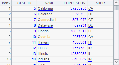
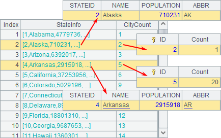
A3 selects the states whose names begin with letter C or any letter after it:

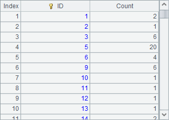
A4 counts the big cities in each state based on the CITIES table:

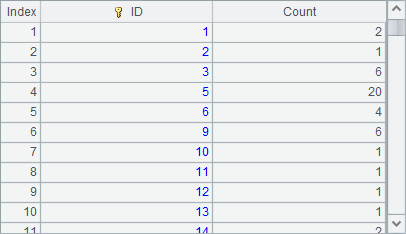
There are two things: A3 doesn’t include the states whose names begin with letter “A” and letter “B” and that the STATEID starts from 6; because not all states have big cities, there are no counts for states whose IDs are 4, 7, 8 and etc. A5 joins the records in A3 and A4 via their state IDs. Result is as follows:

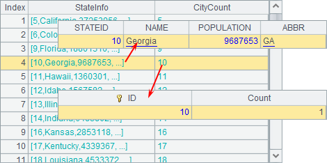
By default, the result of table joins through join function only include records of the two tables whose state IDs can match up. The result can be regarded as a table sequence composed of foreign key fields, each of which references records from the corresponding table.

Generally the join function amounts to the following SQL statement:

–  select A_i.* as F_i,… from A_i,… where A_i.x_j =… and …

That is the most common syntax for a SQL join.

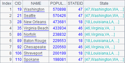
There are other types of joins. For example, join@1 in A6 represents left join. The “1” in option @1 is the number 1 instead of the lowercase letter l, which isn’t used in esProc in case confusion is caused. A6’s result is as follows:

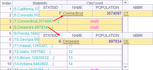
With the left join, all the records of states in A3 are returned to the result, including those that have no matching values in A4, such as the states whose IDs are 7, 8, ….

The join@f in A7 represents the full join. A7’s result is as follows:

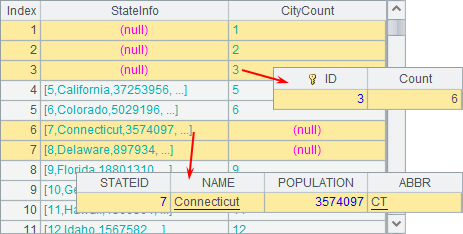
All state records in both A3 and A4 are returned to the result, including some states in A4 that haven’t corresponding values in A3, such as those states whose IDs are 1, 2, 3,…, and some states in A3 that haven’t corresponding values in A4, such as the states with IDs being 7, 8,….

Joining TSeqs by ordinal numbers

It is based on the correspondence of records that join function works to join the references of records in different table sequences. Besides, table sequences can be joined according to record positions. Use @p option to do that. For example:

	A
1	=demo.query("select STATEID,NAME,POPULATION,ABBR from STATES order by STATEID")
2	=demo.query("select * from CITIES")
3	=A2.groups(STATEID:ID;count(~):Count)
4	=join@p(A1:StateInfo;A3:CityCount)

A3 counts big cities in each state based on the CITIES table. Notice that the result lacks the counts for some states:

A4 joins all state records in A1 with the statistical results in A3 according to ordianl numbers and gets the following result:

The number of records in the result is determined by the table sequence with the shorter length. This type of join joins records of two table sequences according to their positions. If the records don’t completely match, you probably get a result where not all records are correctly associated. In the above result, the Arkansas state record, whose ID is 4, is joined mistakenly with the aggregation record of the city count whose ID is 5. In fact, join@p should be used to join tables that have the same length and order:

	A
1	=demo.query("select * from STATENAME")
2	=demo.query("select * from STATECAPITAL")
3	=demo.query("select * from STATEINFO")
4	=join@p(A1:Name;A2:Capital;A3:Info)

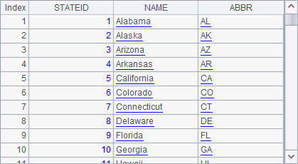
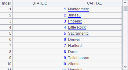
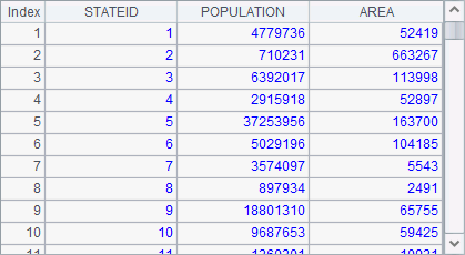
A1, A2 and A3 are respectively a part of all the state information and have the same order:

In this case, they can be joined using join@p, like what A4 does:

The correct result is obtained. For the previous case, the records from the two tables should be joined in alignment using align function.

Cross join

A cross join is a type of join operation that combines each member of the first sequence with each member of the second (or up to n^th) sequence. It is the most basic join operation. Without any filtering condition, it simply lists all possible combinations. xjoin function is used to perform the operation. For example:

	A
1	[1,2,3,4]
2	[a,b,c]
3	=xjoin(A1:Number;A2:Letter)

Result of A3 is as follows:

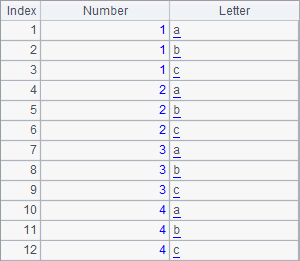
The records in the resulting table sequence are all the possible combinations of the numbers and the letters.

xjoin function can also perform a cross join on records in a table sequence or a record sequence, with one or more filtering conditions specified. For example:

	A
1	=demo.query("select * from STATES")
2	[M,F]
3	=demo.query("select * from EMPLOYEE")
4	=xjoin(A1:State;A2:Gender;A3:Employee,STATE==State.NAME&& GENDER==Gender)

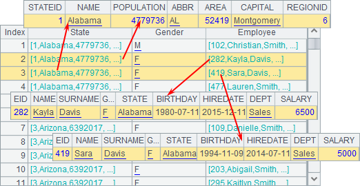
A1 retrieves records of all the states. A2 defines a sequence of genders. A3 retrieves records of all the employees. A4 joins the three sequences by specifying that only the employee records with corresponding state names and genders in A3 are joined. Result of A4 is as follows:

3.5.4 Recursive queries

The foreign key association enables a table sequence to reference records of another table sequence, establishing a pointer type reference relationship between table sequences. You can also make use of the foreign key to perform a self-join in which a table sequence references records in itself to create a hierarchical data structure called a tree. To make data queries in such a tree structure, you need to create recursive queries.

Self-join

Joining a table sequence to itself is like joining multiple table sequences. For example:

	A
1	=file("Geography.txt").import@t()
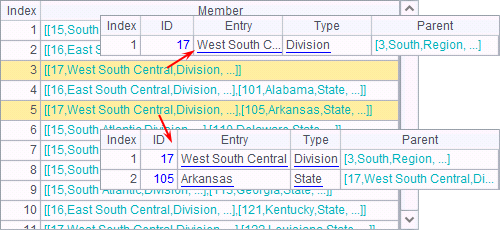
2	>A1.switch(Parent,A1:ID)

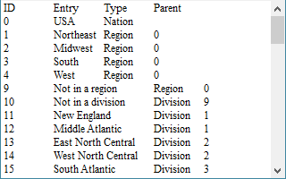
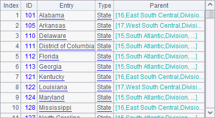
Geography.txt contains information of different levels of places including regions, states, etc. The Parent field shows the code of the parent region of each place. Here’s the original data:

With a self-join, you’ll get the following table:

That is the hierarchical references generated from the self-join.

Recursively querying hierarchical foreign key values for a record

For a hierarchical reference structure produced by a self-join, r.prior(F,r',n) function is used to query every level of data foreign key F of record r references. By specifying r', the function makes a query recursively until the record with referenced record containing the specified value of r' is found in F’s references. The maximum recursion depth n can be set for a recursive query:

	A
1	=file("Geography.txt").import@t()
2	>A1.switch(Parent,A1:ID)
3	=A1.select@1(Entry=="Alabama")
4	=A1.select@1(Entry=="South")
5	=A1.select@1(Entry=="West")
6	=A3.prior(Parent)
7	=A3.prior(Parent,A4)
8	=A3.prior(Parent,A5)

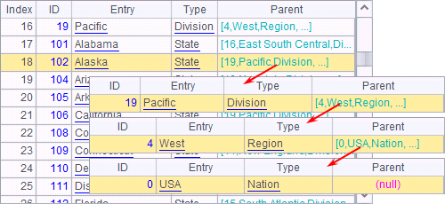
A6 finds all levels of foreign key values the Alabama state record references:

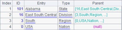
A7 performs recursion until the record containing South is referenced by the Parent value:

A8 returns null because Alabama doesn’t belong to the West region.

Recursively querying children nodes of a given node

prior() function returns records referenced by every level of the foreign key of a record. Conversely, P.nodes(F,r,n) function finds all records referenced under foreign key F in record sequence P. This is equivalent to finding records under record r in a table with hierarchical reference structure. For example:

	A
1	=file("Geography.txt").import@t()
2	>A1.switch(Parent,A1:ID)
3	=A1.select@1(Entry=="South")
4	=A1.nodes(Parent,A3)
5	=A1.nodes@d(Parent,A3)
6	=A1.nodes@p(Parent,A3)

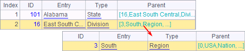
A4 finds records of the states located in South, including the Division level and State level:

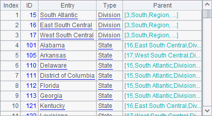
In A5, nodes() function uses @d option to return records without children, where only state records are returned:

In A6, nodes() function uses @p option to return children nodes with their leaf-level nodes, if any, under record r: